This is an age of brute force. Through scaling laws, computation can be traded for gains in capability. Scaling pretraining from millions to billions, and now trillions, of parameters has transformed language and multimodal models. Increasing computation at inference time has further enabled models to reason, search, verify, and tackle increasingly difficult problems.

The tremendous success of brute-force scaling, however, also raises a set of interesting questions. Focusing only on pretraining and fine-tuning, this post touches on a few of them:

Fully answering these questions is obviously challenging. In this blog, we make a more modest argument: the number of parameters, i.e., sizes, is only a coarse measure of capacity; what ultimately matters is how much of that capacity training can exploit. An almost cheating example makes this obvious. Consider exactly the same model, trained for 1K versus 1M iterations. The latter will presumably be much stronger, despite having exactly the same number of parameters — sizes are only part of the story.

But what if we consider a fairer setting, where models are sufficiently well trained? What role does size play in these scenarios? Before getting into concrete examples, here are a few questions that have been on our minds:

• "Large is good" sounds almost too good to be true, or at least too vague to be scientifically satisfying. How large is large? What exactly do we mean by good — training loss, downstream performance, robustness, efficiency, or something else?
• Efficiency still matters. If two models achieve similar performance, we would generally prefer the one that requires fewer parameters, less data, and less computation. Scaling laws tell us that spending more often helps; they do not tell us that spending more is always the most efficient way to improve.

With these questions in mind, this blog uses three real examples to show that increasing model size can, somewhat surprisingly, even hurt performance. Consequently, we argue that the capacity of large models may remain underutilized, and that better exploiting this capacity could make scaling more efficient.

1. A Least-Squares Appetizer

We wanted to go slightly off track with a simple example to build some intuition on why sizes can sometimes hurt. Feel free to jump directly to Section 2 for more realistic problems.

Consider the standard least-squares problem. Let each row of the data matrix $A_m$ correspond to the features of a datum, with the associated labels collected in a vector $b$. Suppose that we only have two data points, and the feature-label pair is defined as

$$A_m = \begin{bmatrix} 1 & 0 & 0 & \cdots & 0 \\ 0 & \frac{1}{m} & \frac{1}{m} & \cdots & \frac{1}{m} \end{bmatrix} \in \mathbb{R}^{2\times(m+1)}, \qquad b = \begin{bmatrix} 1 \\ 1 \end{bmatrix}.$$

The corresponding least-squares problem on an $(m+1)$-dimensional variable is

$$\min_{x_m \in \mathbb{R}^{m+1}} f_m(x_m) = \frac{1}{2}\|A_m x_m - b\|^2.$$

But of course, we can manually redesign the features by merging the last $m$ features into a single one (e.g., feature engineering). In this case, the feature matrix becomes

$$A_1 = \begin{bmatrix} 1 & 0 \\ 0 & 1 \end{bmatrix} \in \mathbb{R}^{2\times 2}, \qquad b = \begin{bmatrix} 1 \\ 1 \end{bmatrix}.$$

We denote the corresponding objective by $f_1(x_1) = \frac{1}{2}\|A_1 x_1 - b\|^2$. Both $f_m$ and $f_1$ describe essentially the same data-fitting problem for the same dataset. The difference lies in the number of parameters: $f_1$ uses only two, whereas $f_m$ uses $m+1$.

Being simple least-squares problems, their optimal solutions are easy to characterize. What is more interesting here is how difficult it is to reach optima using, e.g., gradient descent (GD) with a constant step size $\eta$. What we will show next is that optimizing $f_1$ is easier than $f_m$. And more interestingly, increasing $m$ slows down the convergence of GD — in this example, more parameters lead to slower optimization.

To see this, write $x_m = [u, v_1, \cdots, v_m]^{\top}$. Then we have

$$A_m x_m = \begin{bmatrix} u \\[2mm] \frac{1}{m}\sum_{j=1}^{m} v_j := \bar v \end{bmatrix}.$$

The objective can therefore be rewritten as $f_m(x_m) = \frac12 (u-1)^2 + \frac12 (\bar v - 1)^2$. Clearly, the optimal solution is $u = 1, \bar v = 1$. Let $t$ be the iteration index of GD. Writing out the gradients, it is easily seen that on the first coordinate $u_{t+1} = u_t - \eta(u_t - 1)$, and hence its distance to the optimum satisfies

$$u_{t+1} - 1 = (1-\eta)(u_t - 1) = (1-\eta)^{t+1}(u_0 - 1).$$

For each of the remaining coordinates, $v_{j,t+1} = v_{j,t} - \frac{\eta}{m}(\bar v_t - 1)$. This gives

$$\bar v_{t+1} = \bar v_t - \frac{\eta}{m}(\bar v_t - 1),$$

or equivalently, the distance to the optimum satisfies

$$\bar v_{t+1} - 1 = \left(1 - \frac{\eta}{m}\right)(\bar v_t - 1) = \left(1 - \frac{\eta}{m}\right)^{t+1}(\bar v_0 - 1).$$

Substituting these expressions back into the objective gives an exact characterization of the convergence:

$$f_m(x_{m,t}) = \frac12 (1-\eta)^{2t}(u_0 - 1)^2 + \frac12 \left(1 - \frac{\eta}{m}\right)^{2t}(\bar v_0 - 1)^2,$$

which converges to 0 loss increasingly slowly as $m$ grows. Graphically, Figure 1 validates these derivations.

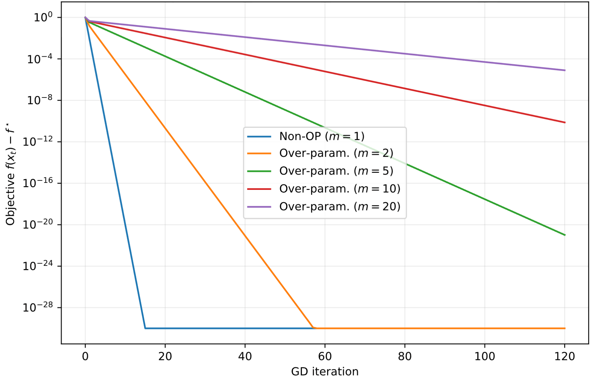
In this example, additional parameters require more iterations to converge. This becomes even more concerning once computational cost is taken into account. Each GD iteration also requires computing a higher-dimensional gradient, and therefore more computation. Taken together, we spend more compute per iteration and more iterations when coping with problems with larger $m$. This simple example already challenges the coarse intuition that a larger parameterization must lead to better outcomes.

2. When Larger Is Not Better: Three Examples in LLMs

While the above example is illustrative, one may reasonably wonder whether the same phenomenon appears in LLMs. In this section, we show that it does: from fine-tuning to pretraining, and from dense to sparsely activated models, larger does not necessarily mean better.

2.1 LoRA fine-tuning does not improve with adapter rank

Our first example comes from low-rank adapters (LoRA), a parameter-efficient approach for fine-tuning LLMs for reduced memory cost. The idea of LoRA fine-tuning, introduced in [1], is to replace the full update of each linear layer with a low-rank Burer–Monteiro factorization. The training objective can be written as

$$\min_{\{A_l, B_l\}_l} f(\{W_l + A_l B_l^\top\}_l)$$

where $f$ is the training loss on the fine-tuning dataset, $W_l \in \mathbb{R}^{m\times n}$ is the $l$-th pretrained weight matrix, and $A_l \in \mathbb{R}^{m \times r}$, $B_l \in \mathbb{R}^{n \times r}$ are trainable LoRA weights. Since the adapter rank $r \ll \min\{m,n\}$, LoRA introduces far fewer trainable parameters than full fine-tuning. For example, with $r=16$ and $m=n=1024$, the LoRA update contains only about $3\%$ as many trainable parameters as full fine-tuning, leading to memory efficiency.

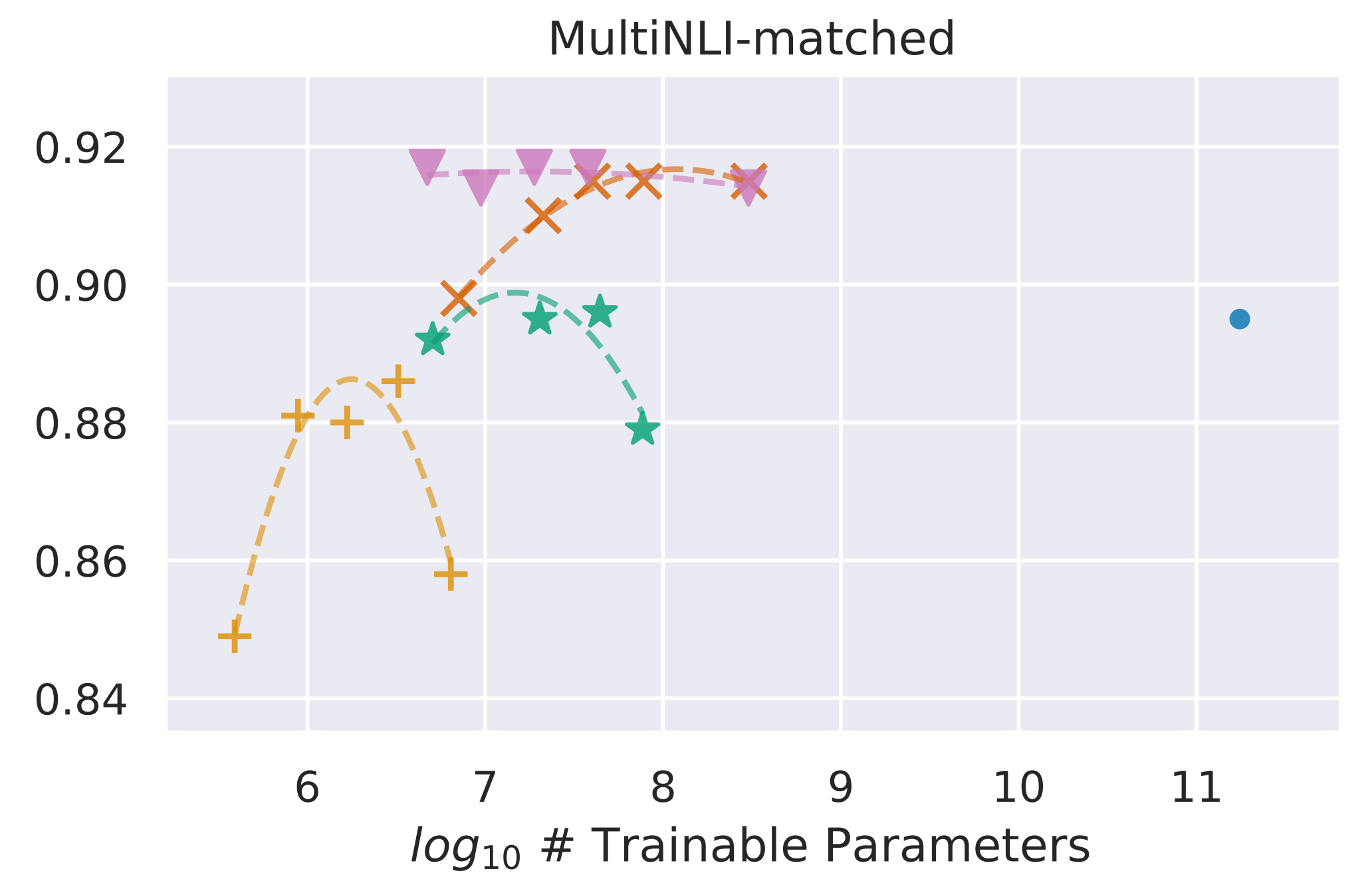
It is natural to expect that, ideally, LoRA performance should not deteriorate as the adapter rank $r$ increases, since a larger rank provides a more expressive update space. In practice, however, this is often not the case. For example, when fine-tuning GPT-3-175B on the MNLI dataset, as shown in Figure 2, LoRA performance can actually drop with a larger $r$. In other words, adding more trainable parameters can make the final model worse.

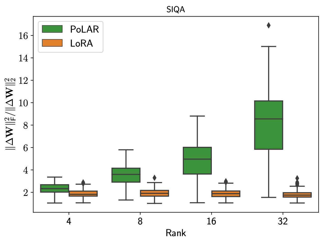
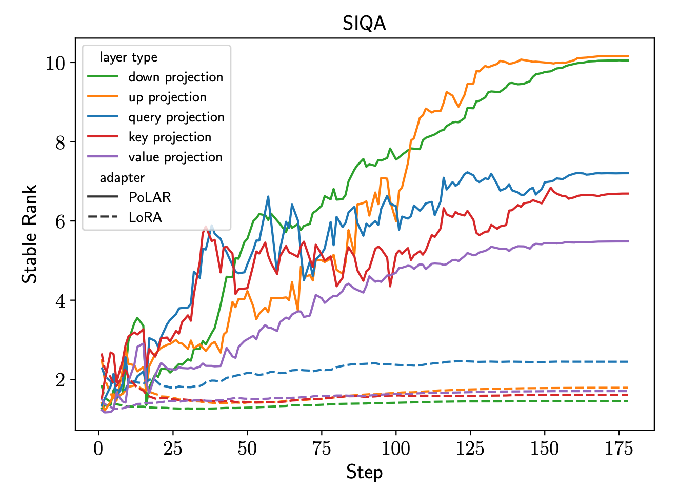
The reason can be seen from Figures 3 and 4 from [2], which analyze the fine-tuning dynamics of LoRA on LLaMA2-7B, used here as a more economical alternative to GPT-3-175B. Figure 3 plots the stable rank, a smooth surrogate for the true rank, of the learned LoRA updates for different adapter ranks $r \in \{4, 8, 16, 32\}$. Surprisingly, the stable rank remains mostly below $2$ across all settings. In the case of $r = 32$, this means that although 32 directions are available in the spectrum, the learned update uses only about two, leaving most of the allocated subspace underutilized. The training dynamics in Figure 4 make this even clearer. The stable rank increases only at the very beginning of fine-tuning and then quickly saturates, showing almost no further growth after roughly $25$ iterations. If the stable rank remains around $2$, allocating a larger $r$ simply introduces more parameters without proportionally increasing the model capacity actually used.

Importantly, the improved performance achieved by another approach, PoLAR [2], together with its higher stable rank, rules out the possibility that a rank-2 solution is already sufficient for good performance. Instead, it suggests that the limitation lies in optimization: as $r$ increases, standard LoRA becomes less effective at exploiting the additional rank from the larger parameterization.

2.2 Deeper LLaMA models do not necessarily learn more nontrivial functions

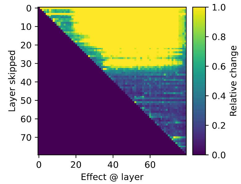
Another example comes from [3], where the authors show that the depth of a pretrained LLaMA 3 model may not be fully utilized. They start from LLaMA 3 70B, which contains 80 Transformer layers, and remove one specific layer, for example, deleting the 5th layer and connecting the 4th and 6th layers. They then feed the same data through the original and modified models and compare the resulting activations layer by layer.

In the corresponding heatmap in Figure 5, brighter pixels indicate larger changes in the activations of the layer-deleted model relative to the original model. The pattern is striking: removing layers before roughly the 40th layer causes substantial downstream changes, whereas removing layers after around the 40th layer has much smaller effects on subsequent activations. Together with the other experiments in the paper, this suggests that a significant fraction of the later layers contribute only small refinements, behaving approximately like identity mappings.

However, an identity mapping is essentially available for free: a feature can simply be passed forward unchanged without any additional transformation. If many of the later layers primarily approximate the identity, in this case, more parameters do not necessarily translate into learning more complicated functions.

2.3 MoE with shared experts may not benefit from more activated parameters

Another setting where larger is not necessarily better appears in mixture-of-experts (MoE) models. Here, by larger, we specifically mean activating more parameters for each token.

MoEs have been instrumental in scaling LLMs to extremely large parameter counts through sparse conditional computation: each token activates only a subset of the available experts, or subnetworks. At the core of an MoE layer is a router and $E$ experts, each typically implemented as a feedforward network (FFN). For each input token, the router selects $K$ experts for sparse activation. Building on this basic design, recent MoEs, such as DeepSeek-v4 and Qwen1.5 MoE, have increasingly adopted two notable architectural advances:

• The first is fine-grained expert segmentation. Recent MoEs tend to use larger numbers of both total and activated experts, i.e., larger $E$ and $K$. For example, at the same activation ratio $K/E$, $(E,K)=(64,8)$ is often preferred over $(E,K)=(8,1)$. Since there are $\binom{E}{K}$ possible expert combinations, larger $E$ and $K$ create a much richer routing space and, in principle, more expressive token representations.
• The second advance is shared experts. Activated for every token, shared experts isolate common knowledge that would otherwise be learned redundantly by routed experts. This allows routed ones to devote more capacity to specialization.

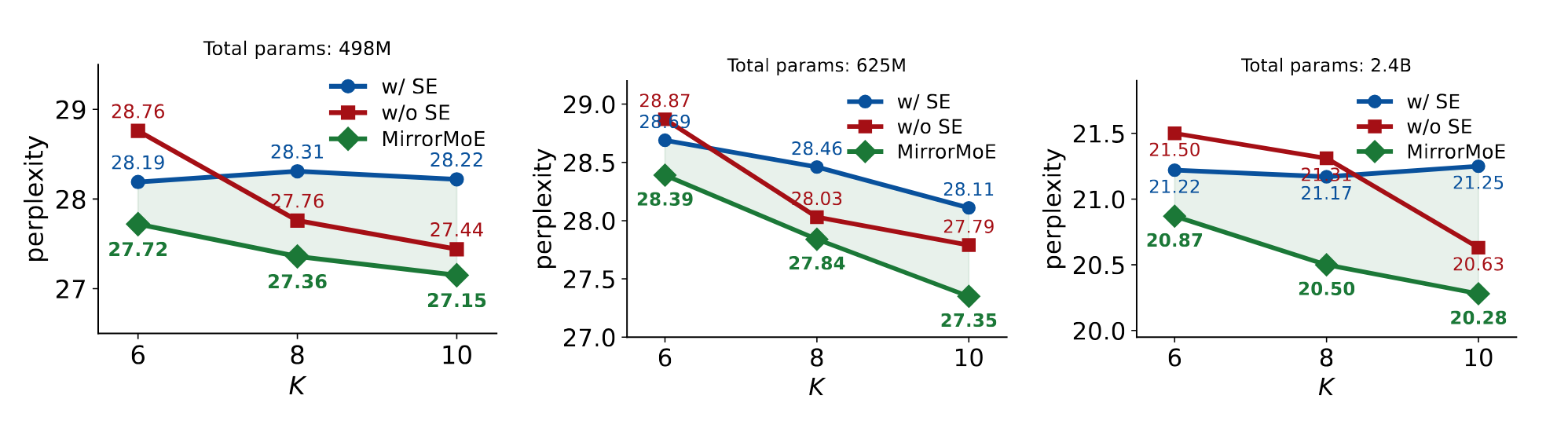
However, a recent study [6] shows that shared experts and fine-grained expert segmentation can compete with each other in terms of routing exploration. We will not go into the technical details here, but this exploration dilemma has tangible consequences for shared-expert MoEs. To illustrate this, [6] trains matched MoE models with and without shared experts across multiple model scales, ranging from hundreds of millions to 2.4B total parameters. At each scale, the total number of experts $E$ is fixed, while the number of activated experts $K$ is varied over $\{6, 8, 10\}$. As shown in Figure 6, for MoEs with shared experts (blue curve), performance can even degrade (larger perplexity) as $K$ increases. In other words, although each token activates more experts, and therefore uses more parameters, the resulting model can actually perform worse.

3. What Does This Mean?

In LoRA, additional rank is available but remains underutilized. In deep Transformers, additional layers may contribute only marginally new computations. In MoEs with shared experts, activating more experts enlarges the routing space, making the additional expressiveness difficult to realize. These messages jointly show that more parameters do not necessarily translate into better performance. In other words, scaling up does not automatically mean scaling better. What scale does bring, however, is cost. More parameters require more computation during training or inference, and, according to data-scaling laws, larger models are often paired with more training data as well. This brings us back to a more fundamental question:

• How can we ensure that additional parameters actually improve performance? Can we design architectures and optimization methods so that newly added capacity is guaranteed to be well-utilized, rather than becoming redundant or difficult to train?
• Are current scaling laws themselves optimal? Scaling laws describe how performance improves as resources increase, but the observed slope is not necessarily optimal. Better architectures, optimization, or utilization of existing capacity may improve the scaling curve itself.

The examples provided in this blog should not be interpreted as arguments against scaling. In fact, several of the issues discussed above can be addressed to make additional parameters genuinely beneficial [2, 3, 4, 5, 6]. Recent work [7] further shows that scaling behavior itself can shift when the same network is optimized differently. Jointly, these results suggest that scaling may still have headroom: future gains in scaling may come not only from making models larger, but also from making each additional parameter easier to optimize and more useful.

References

1. Hu, E. J., Shen, Y., Wallis, P., Allen-Zhu, Z., Li, Y., Wang, S., Wang, L., and Chen, W. "LoRA: Low-rank adaptation of large language models." In ICLR 2022.
2. Lion, K., Zhang, L., Li, B., and He, N. "PoLAR: Polar-decomposed low-rank adapter representation." In NeurIPS 2025.
3. Csordás, R., Manning, C. D., and Potts, C. "Do language models use their depth efficiently?" In NeurIPS 2025.
4. Zhang, Y., Li, B., He, N., and Giannakis, G. B. "ANCRe: Adaptive neural connection reassignment for efficient depth scaling." In NeurIPS 2026.
5. Kimi Team. "Attention residuals." arXiv preprint (2026).
6. Li, B., Ma, H., Muehlebach, M., He, N., and Ma, Y. "Rethinking Routing Exploration in Modern Mixture-of-Experts." arXiv preprint (2026).
7. Jha, N. K., and Reagen, B. "Same Architecture, Different Capacity: Optimizer-Induced Spectral Scaling Laws." arXiv preprint (2026).